Skip to main content
Contents Index Dark Mode Prev Up Next \( {\labelitemi}{$\diamond$}
\def\arraystretch{1.5}
\newcommand{\contentsfinish}{}
\newcommand{\separator}{\begin{center}\rule{\columnwidth}{\arrayrulewidth}\end{center}}
\newcommand{\tosay}[1]{\begin{center}\text{\fbox{\scriptsize{#1}}}\end{center}}
\renewcommand{\cftsecfont}{}
\renewcommand{\cftsecpagefont}{}
\renewcommand{\descriptionlabel}[1]{\hspace{\labelsep}\smallcaps{#1}}
\def\oldequation{\equation}
\def\endoldequation{\endequation}
\newcommand{\nl}{
}
\newcommand{\runin}[1]{\textls[50]{\otherscshape #1}}
\renewcommand{\sectionmark}[1]{}
\renewcommand{\subsectionmark}[1]{}
\renewcommand{\sectionmark}[1]{\markboth{{\thesection}.\ \smallcaps{#1}}{\thesection.\ \smallcaps{#1}}}
\renewcommand{\subsectionmark}[1]{}
\renewcommand{\sectionmark}[1]{\markboth{{\scriptsize\thesection}.\ \smallcaps{#1}}{}}
\renewcommand{\subsectionmark}[1]{}
\newcommand{\makedefaultsection}[2][true]{
}
\newcommand{\timestamp}{{\color{red}Last updated: {\currenttime\ (UTC), \today}}}
\renewcommand{\le}{\leqslant}
\renewcommand{\leq}{\leqslant}
\renewcommand{\geq}{\geqslant}
\renewcommand{\ge}{\geqslant}
\newcommand{\ideal}[1]{\left\langle\, #1 \,\right\rangle}
\newcommand{\subgp}[1]{\left\langle\, #1 \,\right\rangle}
\def\p{\varphi}
\def\isomorphic{\cong}
\def\imp{\to}
\def\iff{\leftrightarrow}
\def\Gal{\text{Gal}}
\def\im{\text{im}}
\def\ran{\text{ran}}
\def\normal{\vartriangleleft}
\renewcommand{\qedsymbol}{$\checkmark$}
\def\lcm{{\text{lcm}\,}}
\newcommand{\q}[1]{{\color{red} {#1}}}
\newcommand{\startimportant}[1]{\end{[{Hint:} #1]\end}}
\renewcommand{\textcircled}[1]{\tikz[baseline=(char.base)]{\node[shape=circle,draw,inner sep=2pt,color=red] (char) {#1};}}
\newcommand{\crossout}[1]{\tikz[baseline=(char.base)]{\node[mynode, cross out,draw] (char) {#1};}}
\newcommand{\set}[1]{\left\{ {#1} \right\}}
\newcommand{\setof}[2]{{\left\{#1\,|\,#2\right\}}}
\def\C{{\mathbb C}}
\def\Z{{\mathbb Z}}
\def\bF{{\mathbb F}}
\def\Q{{\mathbb Q}}
\def\N{{\mathbb N}}
\def\U{{\mathcal U}}
\def\pow{{\mathcal P}}
\def\R{{\mathbb R}}
\newcommand{\h}[1]{{\textbf{#1}}}
\def\presnotes{}
\renewcommand{\d}{\displaystyle}
\newcommand{\N}{\mathbb N}
\newcommand{\B}{\mathbf B}
\newcommand{\Z}{\mathbb Z}
\newcommand{\Q}{\mathbb Q}
\newcommand{\R}{\mathbb R}
\newcommand{\C}{\mathbb C}
\newcommand{\U}{\mathcal U}
\newcommand{\pow}{\mathcal P}
\newcommand{\inv}{^{-1}}
\newcommand{\st}{:}
\renewcommand{\iff}{\leftrightarrow}
\newcommand{\Iff}{\Leftrightarrow}
\newcommand{\imp}{\rightarrow}
\newcommand{\Imp}{\Rightarrow}
\newcommand{\isom}{\cong}
\renewcommand{\bar}{\overline}
\newcommand{\card}[1]{\left| #1 \right|}
\newcommand{\twoline}[2]{\begin{pmatrix}#1 \\ #2 \end{pmatrix}}
\newcommand{\vtx}[2]{node[fill,circle,inner sep=0pt, minimum size=4pt,label=#1:#2]{}}
\newcommand{\va}[1]{\vtx{above}{#1}}
\newcommand{\vb}[1]{\vtx{below}{#1}}
\newcommand{\vr}[1]{\vtx{right}{#1}}
\newcommand{\vl}[1]{\vtx{left}{#1}}
\renewcommand{\v}{\vtx{above}{}}
\newcommand{\lt}{<}
\newcommand{\gt}{>}
\newcommand{\amp}{&}
\definecolor{fillinmathshade}{gray}{0.9}
\newcommand{\fillinmath}[1]{\mathchoice{\colorbox{fillinmathshade}{$\displaystyle \phantom{\,#1\,}$}}{\colorbox{fillinmathshade}{$\textstyle \phantom{\,#1\,}$}}{\colorbox{fillinmathshade}{$\scriptstyle \phantom{\,#1\,}$}}{\colorbox{fillinmathshade}{$\scriptscriptstyle\phantom{\,#1\,}$}}}
\)
Section 6.1 Trees
Worksheet 6.1.1 Worksheet
Guiding Questions. In this section, we’ll seek to answer the questions:
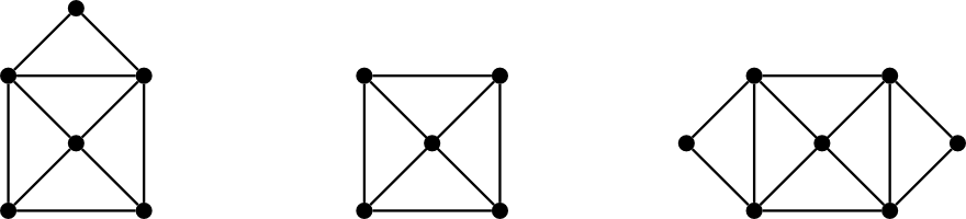
Activity 6.1.1 .
Consider the graphs below.
Figure 6.1.2. Some small graphs.
For each of these graphs, find a subgraph with the smallest number of edges that is still connected and contains all the vertices.
For each of these graphs, find a subgraph with the largest number of edges that does not contain any cycles.
What do you notice about your answers to these questions? What do you wonder?
In this section, we explore certain special classes of graphs. We begin with trees; it may be helpful to review
Definition 5.3.10 .
Definition 6.1.3 .
A
tree is a connected graph which contains no cycles. A
forest is a graph which contains no cycles.
We sometimes also use the word
acyclic to describe trees and forests. Trees are useful structures for modeling decisions, as well as searches. We will return to this notion later. For now, we establish an alternative characterization of trees.
Theorem 6.1.4 .
Suppose
\(T\) is a graph such that between any pair of distinct vertices
\(u,v\) there is a unique path. Then
\(T\) is a tree.
Hint .
First, explain why
\(T\) is connected. Then assume there is a cycle and reach a contradiction.
Theorem 6.1.5 .
Suppose
\(T\) is a tree. Then there is a unique path between any two vertices of
\(T\text{.}\)
Hint .
First, show there is at least one path between any two vertices of
\(T\text{.}\) Then assume that there is a pair of vertices between which there are two paths, and build a cycle to reach a contradiction.
Alternative Characterization of Trees. A graph
\(T\) is a
tree precisely when it is connected and for all pairs of distinct vertices
\(u,v\) in
\(T\) there is a unique path from
\(u\) to
\(v\text{.}\)
We can also make the following observation about forests.
Corollary 6.1.6 .
A graph
\(F\) is a forest if and only if between any pair of vertices in
\(F\) there is at most one path.
We now return to
Activity 6.1.1 to consider a feature of the minimal graphs you produced.
Activity 6.1.7 .
What do you notice? What do you wonder?
A vertex of degree 1 is called a leaf (yes, really). How many leaves does each of your minimal graphs have? Do you think this will always happen? State and prove a conjecture.
Theorem 6.1.8 .
Let
\(T\) be a tree and
\(v\) a leaf of
\(T\text{.}\) Then the graph formed by the removal of
\(v\) and its incident edge,
\(T\setminus v\text{,}\) is a tree.
An important problem in graph theory is the identification of
spanning trees .
Definition 6.1.9 .
Let
\(G = (V,E)\) be a graph and
\(H = (V',E')\) a subgraph of
\(G\text{.}\) We say
\(H\) is a
spanning subgraph if
\(V' = V\) (alternatively, we say that
\(H\) spans \(G\) ). Furthermore, we say that
\(H\) is a
spanning tree of
\(G\) if
\(H\) spans
\(G\) and
\(H\) is also a tree.
Theorem 6.1.10 .
A graph has a spanning tree if and only if it is connected.
A common technique for proving statements about trees is sometimes known as
leaf pruning , and goes hand-in-hand with induction on the number of vertices. At the inductive step, we assume that we have a tree with
\(n+1\) vertices, temporarily
prune one to apply our inductive hypothesis, and then put our
\((n+1)\) st vertex back to reach our conclusion. Try to use this technique to prove the following theorem.
Theorem 6.1.11 .
Let
\(T\) be a tree with
\(v\) vertices and
\(e\) edges. Then
\(e = v - 1\text{.}\)
Theorem 6.1.12 .
Let
\(G\) be a connected graph on
\(v\) vertices. If
\(G\) has
\(v-1\) edges, then
\(G\) is a tree.